Ultimate Guide to Adversarial Regularization
Adversarial regularization is a method that strengthens AI models by training them with adversarial examples - inputs intentionally altered to challenge the model. This approach improves a model's ability to resist attacks and handle subtle variations in input data. Key points include:
- Purpose: Protect AI systems from adversarial attacks that exploit small changes in input data to cause errors.
- Techniques: Includes methods like FGSM (Fast Gradient Sign Method) for quick tests and PGD (Projected Gradient Descent) for more thorough training.
- Benefits: Improves model reliability under challenging conditions without compromising too much on clean data performance.
- Challenges: Balancing robustness with accuracy and managing the added computational demands.
Adversarial regularization uses a min-max optimization framework to train models to minimize their worst-case loss under adversarial conditions. This makes it an essential tool for AI practitioners working in security-sensitive fields or applications requiring consistent performance under diverse conditions.
Core Principles of Adversarial Regularization
Min-Max Optimization Framework
At the heart of adversarial regularization is a min-max optimization framework designed to minimize the worst-case loss instead of the average loss. The formula looks like this:
$ \min_\theta \sum_i \max_{|\delta| \leq \epsilon} \ell\big(h_\theta(x_i + \delta), y_i\big), $
where the inner maximization step identifies the worst-case perturbation (δ) within a constrained norm ball of radius ε. This essentially simulates the strongest adversarial attack possible. The outer minimization then updates the model parameters (θ) to reduce this maximum loss, effectively training the model to resist such adversarial perturbations.
However, solving the inner maximization directly is impractical due to the non-convex nature of loss surfaces. Instead, iterative methods like Projected Gradient Descent (PGD) are used to approximate the worst-case perturbation. For example, a 4-layer deep neural network (DNN) trained on MNIST experienced a dramatic increase in error rate - from 2.1% to 98.38% - when subjected to a PGD attack (ε = 0.1, α = 0.01, 40 iterations).
How Adversarial Examples Work
Adversarial examples are crafted by introducing a small perturbation (δ) to the input (x) that maximizes the model's loss. These changes are typically constrained within an ℓ∞ ball, ensuring that the perturbations (|δ|∞ ≤ ε) remain imperceptible to human eyes. Despite being subtle, these perturbations can drastically alter the model's predictions.
Neural networks are especially vulnerable to such attacks because of their highly irregular loss surfaces. For instance, a ResNet50 model was tricked into classifying an image of a "pig" as an "airliner" with a confidence of 96.8%, even though the image appeared unchanged to human viewers. Interestingly, the average absolute gradient for a single pixel at the starting point (δ = 0) might be as small as 10⁻⁶, but iterative attacks can amplify these gradients enough to flip the model's classification.
During adversarial training, these examples are generated for each minibatch, and the model's weights are updated based on the perturbed data instead of the original clean inputs. This approach is grounded in Danskin's Theorem, which ensures that the gradient of the maximized loss can be computed directly at the point of optimal adversarial perturbation.
These principles form the foundation for adversarial regularization techniques, setting the stage for the methods covered in later sections.
sbb-itb-903b5f2
Lecture 16 | Adversarial Examples and Adversarial Training
Adversarial Regularization Techniques
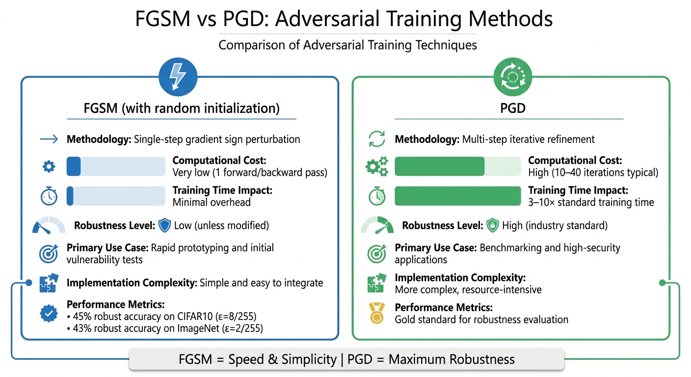
FGSM vs PGD Adversarial Training Methods Comparison
Fast Gradient Sign Method (FGSM)
FGSM is a straightforward and efficient approach for creating adversarial examples. It calculates the gradient of the loss function with respect to the input, then perturbs the input in a single step using the formula:
x_adv = x + ε · sign(∇ₓ J(θ, x, y))
This single-step process makes FGSM highly efficient, particularly for quick vulnerability checks and early-stage testing. However, it has a downside: models trained with FGSM can experience catastrophic overfitting. This means the model may seem resistant to FGSM attacks but remains vulnerable to stronger iterative methods. For example, FGSM with random initialization achieved 45% robust accuracy on CIFAR10 (ε=8/255) and 43% robust accuracy on ImageNet (ε=2/255) while significantly reducing training time compared to other methods.
"Adversarial training with the fast gradient sign method (FGSM), when combined with random initialization, is as effective as PGD-based training but has significantly lower cost." - Eric Wong, Researcher, Locus Lab
While FGSM is excellent for rapid assessments, it lacks the robustness needed for high-stakes scenarios. For such cases, iterative techniques like PGD are more suitable.
Projected Gradient Descent (PGD)
PGD builds on FGSM by refining adversarial perturbations through multiple small steps. After each step, the perturbation is projected back within the ε-boundary, ensuring that changes remain imperceptible. This iterative process makes PGD far more effective at identifying vulnerabilities, although it comes with a much higher computational cost. Typically, PGD requires 10–40 iterations, significantly increasing the time needed for training.
"Adversarial training with the projected gradient decent attack (adv.PGD) is considered as one of the most effective ways to achieve moderate adversarial robustness." - Huang et al.
Despite its resource demands, PGD is widely regarded as the gold standard for evaluating and improving model robustness. Adversarial training with PGD can extend standard training time by 3 to 10 times, but the resulting resilience makes it a preferred choice for critical applications.
Technique Comparison
FGSM and PGD each have strengths and trade-offs, depending on the use case. Here's a side-by-side look at their key features:
| Feature | FGSM (with random initialization) | PGD |
|---|---|---|
| Methodology | Single-step gradient sign perturbation | Multi-step iterative refinement |
| Computational Cost | Very low (1 forward/backward pass) | High (10–40 iterations typical) |
| Training Time Impact | Minimal overhead | 3–10× standard training time |
| Robustness Level | Low (unless modified) | High (industry standard) |
| Primary Use Case | Rapid prototyping and initial vulnerability tests | Benchmarking and high-security applications |
| Implementation Complexity | Simple and easy to integrate | More complex, resource-intensive |
How to Implement Adversarial Regularization
Setting Up the Training Pipeline
Start by building a standard neural network as your baseline. The difference here lies in how you handle the data and configure the loss function. Begin by normalizing input features - like scaling pixel values to a range of 0 to 1. This step is crucial for maintaining numerical stability when calculating gradient-based perturbations.
Next, set the adversarial hyperparameters. These include an adversarial multiplier to weight the loss and a step size to control the magnitude of perturbations. You’ll also need to select a norm, typically either L∞ or L₂, to measure the size of the perturbations.
To evaluate your model, implement a dual-evaluation setup. This involves testing performance on both clean and adversarial inputs. This approach ensures your model remains accurate on normal data while showing resilience under adversarial conditions.
The next step focuses on generating adversarial examples, which simulate attack scenarios.
Generating Adversarial Examples
Once your pipeline is ready, the focus shifts to crafting adversarial inputs using gradients. During training, you’ll create these examples by flipping the usual training logic. Instead of minimizing the loss by adjusting model weights, you maximize the loss by tweaking the input data using backpropagated gradients. Start by enabling input gradients by setting requires_grad to true before the forward pass.
For methods like FGSM (Fast Gradient Sign Method), calculate the gradient of the loss with respect to the input and perturb the input in a single step. For PGD (Projected Gradient Descent), take multiple smaller steps and project the perturbed inputs back into the epsilon-ball (a defined range of allowable perturbations). Always clip the perturbations to ensure the inputs remain valid. When using PGD, set the step size (α) to a small fraction of the total epsilon (ε) and ensure the number of iterations aligns with ε/α.
"Rather than working to minimize the loss by adjusting the weights based on the backpropagated gradients, the attack adjusts the input data to maximize the loss based on the same backpropagated gradients." - Nathan Inkawhich, Author
Testing and Tuning Model Performance
Once adversarial examples are generated, thorough testing is essential to confirm the model’s robustness against varying levels of attack intensity. This involves evaluating performance across a range of perturbation strengths rather than just one epsilon value. Plotting robustness curves can reveal how accuracy changes as the strength of the attack increases. Ideally, with proper regularization, your model can maintain robust accuracy at around 95-96%, while clean data accuracy stays close to 99%.
Fine-tuning your model requires careful adjustment of two key hyperparameters: the adversarial multiplier (which controls the weight of adversarial loss) and the adversarial step size (which determines the size of perturbations). Increasing the multiplier can improve robustness but might slightly lower clean accuracy. If fine-tuning a pre-trained model, lower the learning rate - dropping from 1e-3 to 1e-4, for instance - to stabilize training. Use mixed batches with a 50/50 split of normal and adversarial examples. This helps the model learn to defend against its own generated adversarial inputs.
Be vigilant for gradient masking, where the model appears robust because it flattens its gradients, making it difficult for gradient-based attacks to succeed. However, such a model might still be vulnerable to other attack types. Always inspect adversarial examples manually to ensure perturbations are subtle enough to remain undetectable to human eyes. If the altered image is unrecognizable, your epsilon value is likely too high.
Benefits, Challenges, and Best Practices
Benefits of Adversarial Regularization
Adversarial regularization offers several practical advantages. It helps models generalize better by avoiding the pitfalls of overfitting and learning irrelevant noise. This means the models are more reliable when faced with new, unseen inputs. Additionally, they become more adept at identifying and addressing vulnerabilities before deployment.
The security advantages are especially critical in high-stakes fields like autonomous driving, biometric authentication, and healthcare diagnostics. These areas are particularly vulnerable to malicious perturbations. For instance, standard models can lose nearly half their accuracy during an attack, while adversarial regularization helps maintain performance levels. The urgency for such defenses is clear, given the 35% rise in detected adversarial attacks on AI models in 2025.
Common Challenges and Solutions
Despite its promise, adversarial regularization comes with its own set of challenges. One major hurdle is the robustness–accuracy trade-off. Strengthening a model's resistance to attacks often diminishes its performance on clean, unaltered data. For example, heavy adversarial training can lower helpfulness scores (from 4.5 to 3.2) and increase over-refusal rates (from 0.5% to 12%). To address this, careful optimization of the adversarial mix ratio - keeping it between 15–30% in training batches - can help strike a balance between robustness and overall performance.
Another challenge is the computational cost. Adversarial training can be resource-intensive; training on ImageNet using a 10-step PGD method, for instance, takes about six days on 4 V100 GPUs, compared to just two hours on a single GPU for CIFAR-10 training. Techniques like Split-BatchNorm (Split-BN), which uses separate Batch Normalization layers for clean and adversarial inputs, can help manage these computational demands. Additionally, adding a small predictor MLP head can improve stability by smoothing updates and reducing gradient norms during training.
These challenges highlight the importance of adopting targeted strategies to ensure effective implementation.
Best Practices
To get started, run small-scale experiments with a low adversarial mix ratio (5–15%) to observe how it impacts model performance. Use validation datasets to measure both robustness (e.g., Attack Success Rate) and overall capability (e.g., Factual Accuracy and Instruction Following) on test sets. When fine-tuning, consider lowering the learning rate - dropping from 1e-3 to 1e-4 can help stabilize training and prevent catastrophic forgetting. Limiting training to 1–3 epochs is also a good way to avoid overfitting to adversarial patterns.
Pairing adversarial regularization with Stochastic Weight Averaging (SWA) can enhance generalization and overall model performance. Be vigilant for gradient masking by testing the model against various attack types, not just gradient-based ones. Finally, maintain a continuous training loop that incorporates new adversarial examples from production environments. This ensures your model stays prepared for evolving threats.
Conclusion
Summary of Key Concepts
Adversarial regularization provides models with the resilience needed to handle subtle manipulations that could otherwise cause significant performance issues. Using a min-max optimization framework, this method counters adversarial attacks by crafting challenging examples during training. Techniques like FGSM (a quick, single-step approach) and PGD (a widely recognized iterative method) are central to this process. Among all approaches, adversarial training - where models learn from both clean and adversarial examples - proves to be the most effective defense. Adjusting hyperparameters carefully is crucial to strike the right balance between a model's robustness and accuracy. These principles form the foundation for developing models that can endure real-world adversarial challenges.
Final Thoughts
This guide breaks down the complexities of adversarial regularization, offering practical steps to protect AI systems in increasingly challenging environments. Robust adversarial training isn't just a theoretical concept; it's an essential practice. The urgency is underscored by projections showing a 35% rise in detected adversarial attacks on AI models by 2025. Neglecting these vulnerabilities could jeopardize critical systems. In areas like autonomous vehicles and biometric security, even one misclassification could lead to severe repercussions. Studies reveal that models properly trained with adversarial methods can achieve 96.41% accuracy on adversarial examples, compared to a mere 1.88% accuracy in unprotected models. Starting with lower adversarial mix ratios and testing against varying attack strengths is a practical way to begin. Establishing a continuous training loop that integrates new threats from production environments ensures that defenses remain effective. These strategies provide actionable steps to fortify AI systems against adversarial risks today.
FAQs
How do I choose a good epsilon value?
Choosing the right epsilon value means finding a balance where the perturbations effectively test the model without introducing unrealistic changes. Adaptive approaches, such as learnable dynamic epsilon scheduling, can fine-tune epsilon for each sample and iteration. This adjustment often considers factors like the gradient norm and the model's confidence. It's best to begin with a small, barely noticeable epsilon and fine-tune it using metrics that measure both performance and robustness. This helps avoid values that are either too insignificant or overly disruptive.
When should I use FGSM vs PGD?
FGSM (Fast Gradient Sign Method) is perfect when you need fast and computationally light adversarial examples. It’s a single-step approach that tweaks the input using the sign of the gradient, making it ideal when speed is a priority, even if the perturbations are slightly more noticeable.
On the other hand, PGD (Projected Gradient Descent) is your go-to for creating stronger, harder-to-detect adversarial examples. Its iterative nature allows it to refine the attack over multiple steps, making it especially useful for adversarial training and testing defense mechanisms. This method is better suited for generating robust, worst-case scenarios.
How can I detect gradient masking?
Gradient masking can be identified by evaluating the model with different types of adversarial attacks, particularly those that don't depend on gradient information. Examples include black-box attacks or iterative methods. If the model withstands gradient-based attacks but succumbs to these alternative methods, it could suggest the presence of masking. Another approach is to examine the gradients themselves - indicators like unusually small or noisy gradient values can reveal whether the model's robustness is genuine or simply a result of masking.